Bayesian multivariate inverse variance weighted model with a choice of prior distributions fitted using RStan.

Bayesian multivariate inverse variance weighted model with a choice of prior distributions fitted using RStan.

mvmr_ivw_stan(
  data,
  prior = 1,
  n.chains = 3,
  n.burn = 1000,
  n.iter = 5000,
  seed = 12345,
  ...
)

Arguments

data	A data of class mvmr_format.
prior	An integer for selecting the prior distributions; 1 selects a non-informative set of priors; 2 selects weakly informative priors; 3 selects a pseudo-horseshoe prior on the causal effect.
n.chains	Numeric indicating the number of chains used in the HMC estimation in rstan, the default is 3 chains.
n.burn	Numeric indicating the burn-in period of the Bayesian HMC estimation. The default is 1000 samples.
n.iter	Numeric indicating the number of iterations in the Bayesian MCMC estimation. The default is 5000 iterations.
seed	Numeric indicating the random number seed. The default is 12345.
...	Additional arguments passed through to rstan::sampling().

Value

An object of class stanfit.

References

Burgess, S., Butterworth, A., Thompson S.G. Mendelian randomization analysis with multiple genetic variants using summarized data. Genetic Epidemiology, 2013, 37, 7, 658-665 doi: 10.1002/gepi.21758 .

Stan Development Team (2020). "RStan: the R interface to Stan." R package version 2.19.3, https://mc-stan.org/.

Examples

# \donttest{
if (requireNamespace("rstan", quietly = TRUE)) {
dat <- mvmr_format(rsid = dodata$rsid,
          xbeta = cbind(dodata$ldlcbeta,dodata$hdlcbeta,dodata$tgbeta),
          ybeta = dodata$chdbeta,
          xse = cbind(dodata$ldlcse,dodata$hdlcse,dodata$tgse),
          yse = dodata$chdse)
mvivw_fit <- mvmr_ivw_stan(dat)
print(mvivw_fit)
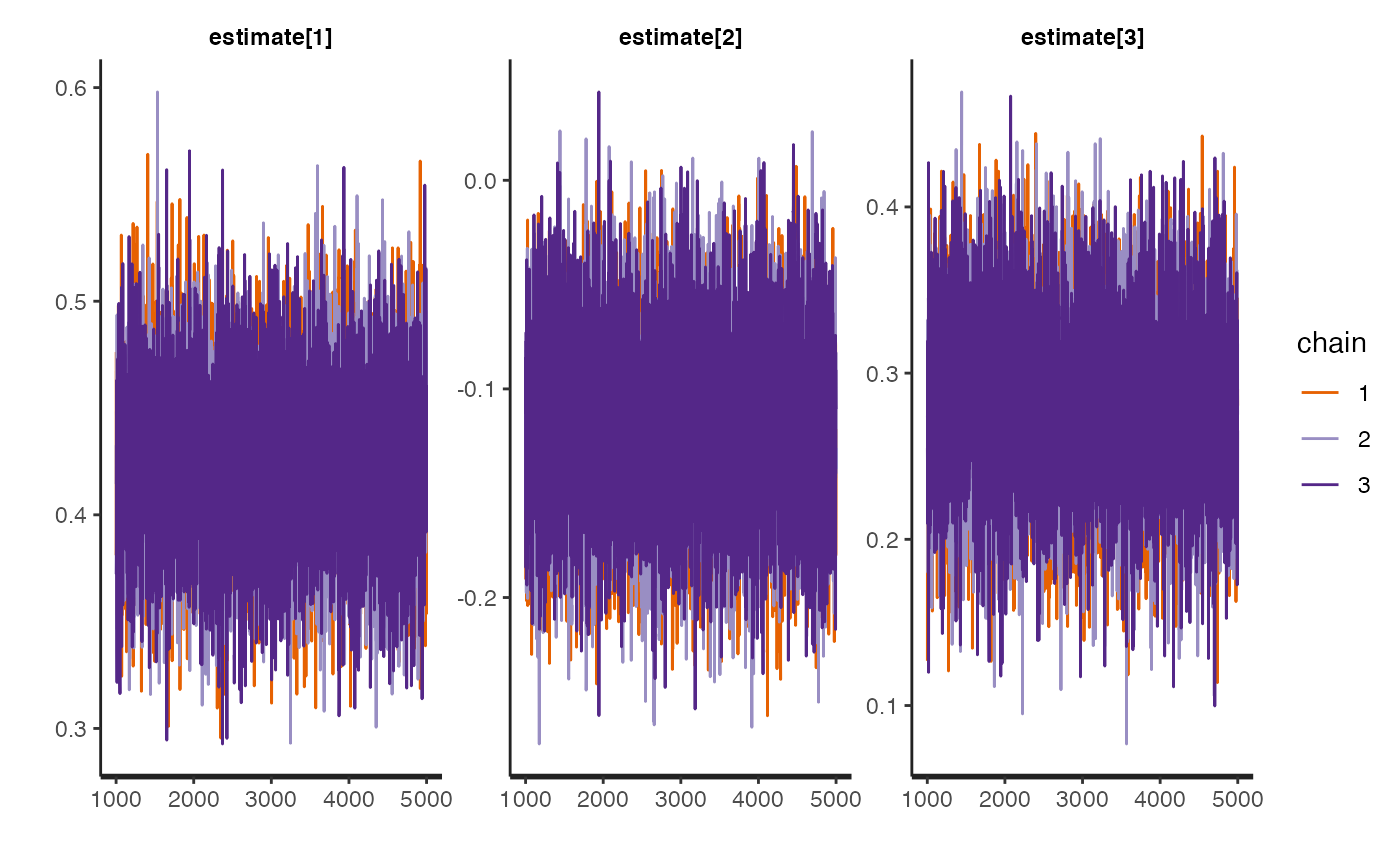
rstan::traceplot(mvivw_fit)
}
#> Inference for Stan model: mvmrivw.
#> 3 chains, each with iter=5000; warmup=1000; thin=1; 
#> post-warmup draws per chain=4000, total post-warmup draws=12000.
#> 
#>                mean se_mean   sd    2.5%     25%     50%     75%   97.5% n_eff
#> estimate[1]    0.42    0.00 0.04    0.35    0.40    0.42    0.45    0.50  6505
#> estimate[2]   -0.12    0.00 0.04   -0.20   -0.15   -0.12   -0.09   -0.04  6596
#> estimate[3]    0.28    0.00 0.05    0.18    0.25    0.28    0.31    0.38  6174
#> lp__        -198.11    0.02 1.23 -201.39 -198.66 -197.78 -197.21 -196.73  4664
#>             Rhat
#> estimate[1]    1
#> estimate[2]    1
#> estimate[3]    1
#> lp__           1
#> 
#> Samples were drawn using NUTS(diag_e) at Thu Oct  7 10:00:41 2021.
#> For each parameter, n_eff is a crude measure of effective sample size,
#> and Rhat is the potential scale reduction factor on split chains (at 
#> convergence, Rhat=1).
# }