Bayesian multivariate inverse variance weighted model with a choice of prior distributions fitted using JAGS.

Usage

mvmr_ivw_rjags(
  object,
  prior = "default",
  betaprior = "",
  n.chains = 3,
  n.burn = 1000,
  n.iter = 5000,
  seed = NULL,
  ...
)

Arguments

object

A data object of class mvmr_format.

prior

A character string for selecting the prior distributions;

"default" selects a non-informative set of priors;
"weak" selects weakly informative priors;
"pseudo" selects a pseudo-horseshoe prior on the causal effect.

betaprior

A character string in JAGS syntax to allow a user defined prior for the causal effect.

n.chains

Numeric indicating the number of chains used in the MCMC estimation, the default is 3 chains.

n.burn

Numeric indicating the burn-in period of the Bayesian MCMC estimation. The default is 1000 samples.

n.iter

Numeric indicating the number of iterations in the Bayesian MCMC estimation. The default is 5000 iterations.

seed

Numeric indicating the random number seed. The default is the rjags default.

...

Additional arguments passed through to rjags::jags.model().

Value

An object of class mvivwjags containing the following components:

CausalEffect: The mean of the simulated causal effects
StandardError: Standard deviation of the simulated causal effects
CredibleInterval: The credible interval for the causal effect, which indicates the lower (2.5%), median (50%) and upper intervals (97.5%)
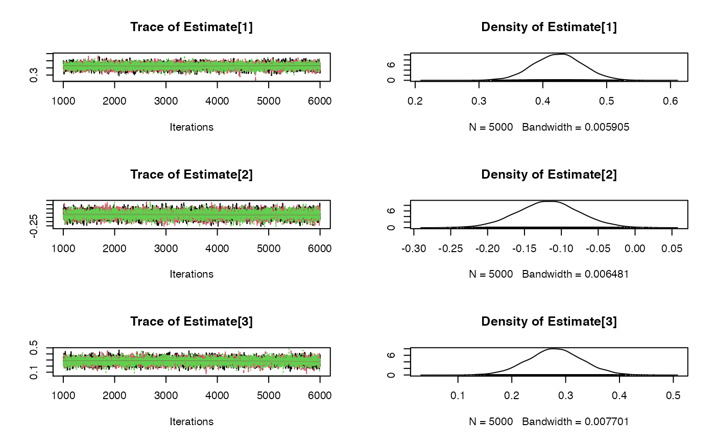
samples: Output of the Bayesian MCMC samples with the different chains
Priors: The specified priors

References

Burgess, S., Butterworth, A., Thompson S.G. Mendelian randomization analysis with multiple genetic variants using summarized data. Genetic Epidemiology, 2013, 37, 7, 658-665 doi:10.1002/gepi.21758 .

Examples

if (requireNamespace("rjags", quietly = TRUE)) {
dat <- mvmr_format(
  rsid = dodata$rsid,
  xbeta = cbind(dodata$ldlcbeta,dodata$hdlcbeta,dodata$tgbeta),
  ybeta = dodata$chdbeta,
  xse = cbind(dodata$ldlcse,dodata$hdlcse,dodata$tgse),
  yse = dodata$chdse
)

fit <- mvmr_ivw_rjags(dat)
print(fit)
summary(fit)
plot(fit$samples)
# 90% credible interval
fitdf <- do.call(rbind.data.frame, fit$samples)
cri90 <- sapply(fitdf, quantile, probs = c(0.05, 0.95))
print(cri90)
}
#>                  Estimate         SD       2.5%        50%      97.5%
#> Causal Effect1  0.4235412 0.03836709  0.3484561  0.4233091  0.4985763
#> Causal Effect2 -0.1171498 0.04195474 -0.2000855 -0.1170895 -0.0361604
#> Causal Effect3  0.2807476 0.05077301  0.1814942  0.2805495  0.3809082
#> Prior : 
#> 
#>  for (j in 1:K) {
#>   Estimate[j] ~ dnorm(0,1E-3)
#>   } 
#> 
#> Estimation results: 
#>  
#>  MCMC iterations = 6000 
#>  Burn in = 1000 
#>  Sample size by chain = 5000 
#>  Number of Chains = 3 
#>  Number of SNPs = 185 
#>  
#>                  Estimate         SD       2.5%        50%      97.5%
#> Causal Effect1  0.4235412 0.03836709  0.3484561  0.4233091  0.4985763
#> Causal Effect2 -0.1171498 0.04195474 -0.2000855 -0.1170895 -0.0361604
#> Causal Effect3  0.2807476 0.05077301  0.1814942  0.2805495  0.3809082

#>     Estimate[1] Estimate[2] Estimate[3]
#> 5%    0.3604705 -0.18676371   0.1967331
#> 95%   0.4874204 -0.04946738   0.3641892